Estimating P2P Overlay Properties: Bittorrent
Mohamad Dikshie Fauzie
Graduate School of Media and Governance
Keio University, 252-0882 Kanagawa, Japan
dikshie@sfc.wide.ad.jp
This report describes an experimental study of the overlay topologies of real-world P2P networks: Bittorrent, focusing on the
activity of the nodes of its P2P topology and especially their dynamic relationships. Peer Exchange Protocol (PEX) messages
are analyzed to infer topologies and their properties, capturing the variations of their behavior. Our measurements, verified using
the Kolmogorov-Smirnov goodness of fit test and the likelihood ratio test and confirmed via simulation, show that a power-law
with exponential cutoff is a more plausible model than a pure power-law distribution. We also found that the average clustering
coefficient is very low, supporting this observation. Bittorrent swarms are far more dynamic than has been recognized previously,
potentially impacting attempts to optimize the performance of the system as well as the accuracy of simulations and analyses.
I. Introduction
Among P2P applications, Bittorrent is the most popular. In 2008, P2P transfer dominated Internet traffic and Bittorrent is the most
popular P2P protocol. P2P traffic is still growing, though recent studies suggest that its growth is slower than that of Internet traffic as a
whole [1] [2].
Many properties of Bittorrent, such as upload/download performance and peer arrival and departure processes, have been studied
[3], but only a few projects have assessed the topological properties of Bittorrent. The Bittorrent system is different from other P2P
systems. The Bittorrent protocol does not offer peer traversal and the Bittorrent tracker also does not know about topologies since peers
never send information to the tracker concerning their connectivity with other peers. While a crawler can be used in other P2P
networks, such as Gnutella, in Bittorrent we cannot easily use a crawler to discover topology, making direct measurement of the
topology difficult.
In this paper we describe our study of Bittorrent networks, where real-world Bittorrent swarms were measured using a
rigorous and simple method in order to understand the Bittorrent network topology. To our knowledge, our approach is
the first to perform such a study on real-world Bittorrent network topologies. We used the Bittorrent Peer Exchange
(PEX) messages to infer the topology of Bittorrent swarms listed on a Bittorrent tracker claiming to be the largest
Bittorrent network on the Internet [4] [5], instead of building small Bittorrent networks on testbeds such as PlanetLab
and OneLab as other researchers have done. We also performed simulations using the same approach to show the
validity of the inferred topology resulted from the PEX messages by comparing it with the topology of the simulated
network.
In addition to demonstrating the validity of our measurement methods, we show that a power-law with exponential cut-off
distribution is a better model than a pure power-law distribution. In terms of the clustering property, we show Bittorrent networks is
more of a random network than a scale-free network. While these results may contradict earlier findings, our simulations also
demonstrated the same phenomenon.
The rest of this paper is organized as follows. We first briefly explain the Bittorrent PEX, followed by the experiment methodology to
infer Bittorrent network topologies using PEX. In the analysis, this paper looks into the power-law distribution and an alternative
distribution to power-law. This paper also inspects the clustering property.
II. Bittorrent Peer Exchange
Bittorrent is a P2P application designed to distribute large files with a focus on scalability and efficiency. When joining a swarm, a
Bittorrent application contacts a tracker, which responds with an initial peer set of randomly selected peers, possibly including seed and
leecher IP addresses and port numbers.
PEX is a mechanism introduced in Bittorrent to discover other peers in the swarm, in which two connected peers exchange messages
containing a set of connected peers. With PEX, peers only need to use the tracker as an initial source of peers. Based on a
survey by the authors of several Bittorent client web sites, it appears that most clients began to introduce PEX in 2007
[6].
However, there is no PEX specification, only a kind of informal understanding among Bittorrent client developers. Therefore there
are differences, e.g., for some Bittorrent clients derived from rasterbar libtorrent [7], the PEX message can only contain a
maximum of a hundred IP address and port pairs. In other Bittorrent clients, the number of IP address and port pairs is
decided based on the size of the PEX message. This implementation difference may affect the ultimate behavior of the
network.
III. Methodology and Experiment Design
We used PEX to collect peer neighbors information (see Figure 1) and then we describe the network formed in terms of properties
such as node degree and average clustering. Besides collecting data from real Bittorrent networks, we ran simulations similar to these of
Al-Hamra et al. [8]. In these simulations, we assumed that peer arrivals and departures (churns) follow an exponential distribution as
explained by Guo et al. [3]. For simplification, we assumed that nodes are not behind a NAT. Since we are only interested in
the construction of the overlay topology, we argue that our simulations are thorough enough to explain the overlay
properties.
Temporal graphs have recently been proposed to study real dynamic graphs, with the intuition that the behaviour of dynamic
networks can be more accurately captured by a sequence of snapshots of the network topology as it changes over time. An
instantaneous snapshot is taken at an exact time point thus capturing only a few nodes and links. In this paper, we study the network
dynamics by continously taking network snapshots with the duration τ as time evolves, and show them as a time series. A snapshot
captures all participating peers and their connections within a particular time interval, from which a graph can be generated. The
snapshot duration may have minor effects on analyzing slowly changing networks. However, in a P2P network, the
characteristics of the network topology vary greatly with respect to the time scale of the snapshot duration to be the
mentioned in [9]. We consider τ = 3 minutes to be a reasonable estimate of minimum session length in the Bittorrent
[10].
A. Graph Sampling
Suppose that a Bittorrent overlay network is a graph G(V,E) with the peers or nodes as vertices and connections between the peers
as edges. If we observe the graph in a time series, i.e., we take samples of the graph, the time-indexed graph is Gt = G(Vt,Et). We
define a measurement window [t0,t0 +Δ] and select peers at random from the set:
 | (1) |
Stutzbach et al. [11] showed that Equation (1) is only appropriate for exponentially distributed peer session lengths and as we know
from existing measurements Bittorrent networks peer session lengths have very high variation [3]. Equation 1 focuses on sampling
peers instead of peer properties. To cope with that problem we must be able to sample from the same peer more than once at different
points in time [11]. We may rewrite our desired sample as
![vi,t ∈ Vt,t ∈ [t0,t0+ Δ].](mori2x.png) | (2) |
The number of peers in a swarm that is observed by our client is our population. The sampled peers set is the number of peers that
exchange PEX messages with our client. Our sampled peers set through PEX messages exchange can observe about 70% of the peers
in a population. This observation is consistent with [12].
B. Experimental Methodology
We crawled top 35 TV series torrent from the piratebay, which claims to be the biggest torrent tracker on the Internet. Our nodes
used a modified Rasterbar libtorrent[14], which is the most popular library. We modified rasterbar’s libtorrent client to become
connection greedy, i.e., try to connect to every peer about whom it received information from the tracker and other peers, remove the
connection limit, and log PEX messages received from other clients. PEX messages sent from old versions of Vuze Bittorrent client
contain not only currently connected peers but also its historically connected peers. We can distinguished Vuze Bittorrent
clients from the log files. To cope with this situation, we do not include old Vuze client in data processing. Removal of
some peers in data processing is valid in terms of sampling with dynamics, see equation 2. We also study the source
code of two popular Bittorrent clients, uTorrent (using rasterbar libtorrent source code) and Vuze, in term of peer
connectivity. Both clients by default try to connect to node candidates randomly without any preference thus we have random
data sets. It implies that our data set is independent to measurement location and a limited number of measurement
locations.
C. Data Analysis Background
Many realistic networks exhibit the scale-free property [13], though we note that “scale-free” is not a complete description of a
network topology [14] [15]. It has been suggested that Bittorrent networks also might have scale-free characteristics [16]. In this
paper, we test this hypothesis.
In a scale-free network, the degree distribution follows a power-law distribution. A power-law distribution is quite a natural model
and can be generated from simple generative processes [17], and power-law models appear in many areas of science [13]
[17].
A power-law distribution can be described as
![Pr[X ≥ x]∝ cx-α.](mori4x.png) | (3) |
where x is the quantity of distribution and α is commonly called the scaling parameter. The scaling parameter usually lies in the range
1.8 < α < 3.5. In discrete form, the above formula can be expressed as:
 | (4) |
This distribution diverges on zero, therefore there must be a lower bound of x called xmin > 0 that holds for the sample to be
fitted by a power-law. If we want to estimate a good power-law scaling parameter then we must also have a good xmin
estimation.
We use maximum likelihood to estimate the scaling parameter α of power-law as described detail in [13]. This approach is accurate
to estimate the scaling parameter in the limit of large sample size. For the detailed calculations of both xmin and alpha, see Appendix B
in [13].
IV. Experiment Results
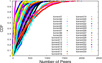
The CDF of the number of peers for every swarm during measurement show in figure 2. It is clear that the number of peers has high
variability due to churn in Bittorrent networks.
A. Power-law Distribution of Node Degree
We want to know the power-law distribution of the measured Bittorrent networks, and we do not know a priori if our data are
power-law distributed. Simply calculating the estimated scaling parameter gives no indication of whether the power-law is
a good model. To test the applicability of a power-law distribution, we use the goodness-of-fit test as described by
Clauset et al. [13]. First, we fit data to the power-law model and calculate the Kolmogorov-Smirnov (KS) statistic
for this fit. Second, we generate power-law synthetic data sets based on the scaling parameter α estimation and the
lower bound of xmin. We fit the synthetic data to a power-law model and calculate the KS statistics, then count what
fraction of the resulting statistics is larger than the value for the measured data set. This fraction is called the p value. If
p ≥ 0.1 then a power-law model is a good model for the data set and if p < 0.1 then power-law is not a good model
[13].
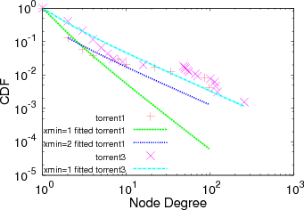
As mentioned before, a good estimation for xmin is important to get a overall good fit. Too small an xmin will cause a fit only to the
body of the distribution. Too high an xmin will cause a fit only to the tail of the distribution. Figure 3 shows the fitting problem example
for data set torrent1 and torrent3. In torrent1 the optimum xmin = 2 and α = 2.11 if we put xmin = 1 we will get α = 2.9 and the fit
visually seems not good, while in the same graph we also show the optimum xmin = 1 for torrent3 and the fit visually seems
good.
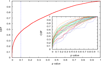
Figure 4 shows the CDF for p values for all data sets. This figure shows that from the K-S statistics point of view around 45% of the
time of Bitorrent networks do not follow a power-law model at any given point in time.
However these data sets must be interpreted with care. The usage of the maximum likelihood estimators for parameter estimation in
power-law is guaranteed to be unbiased only in the asymptotic limit of large sample size, and some of our data sets fall below the rule
of thumb for sample size n = 50 [13]. Also, for the goodness-of-fit test, a large p value does not mean the power-law is the correct
distribution for data sets, because there may be other distributions that match the data sets and there is always a possibility that small
value of p the distribution will follow a power-law even though the power-law is not the right model [13]. We address these concerns
next.
B. Alternative Distributions
Even if we have estimated the power-law parameter properly and the fit is decent, it does not mean the power-law
model is good. It is always possible that non power-law models are better than the power-law model. We use the
likelihood ratio test [18] to see whether other distributions can give better parameter estimation. We only consider
a power-law model and a power-law with exponential cut-off model as examples to show model selection. Model
selection for power-law model and power-law with exponential cut-off is a kind of nested model selection problem.
In a nested model selection, there is always the possibility that a bigger family (power-law) can provide as good a
fit as the smaller family (power-law with exponential cut-off). Vuong [18] provides foundation of the significance
value (ρ value) for likelihood ratio test. For concrete explanation and real-world examples, we refer the readers to
[13].
Under the likelihood ratio test, we compare the pure power-law model to power-law with exponential cut-off, and the ρ value here
helps us establish which of three possibilities occurs: (i) ρ > 0.1 means there is no significant difference between the likelihood of the
data under the two hypotheses being compared and thus neither is favored over the other; if we already rejected the pure
power-law model, then this does not necessarily tell us that we also can reject the alternative model; (ii) ρ < 0.1 and sign
of loglikelihood ratio = negative means that there is a significant different in the likelihoods and that the alternative
model is better; if we have already rejected the pure power-law model, then this case simply tells us that the alternative
model is better than the bad model we rejected; (iii) if ρ < 0.1 and sign of loglikelihood ratio = positive means that
there is a significant difference and that the pure power-law model is better than the alternative; if we have already
rejected the pure power-law model, then this case tells us the alternative is even worse than the bad model we already
rejected.
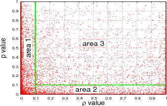
Figure 5 shows a scatter plot of our data: p value vs ρ value. We divide the figure into three areas: area 1, area 2, and area 3. Area
1: ρ value < 0.1 and p value > 0. Area 2: ρ value > 0.1 and p value < 0.1 Area 3: ρ value > 0.1 and p value > 0.1 This division will
make us easier to see how sparse the points are in each area and to see how many points fall into ρ value < 0.1. For points in area 1,
an alternative model may be plausible for data sets. In this figure we do not include loglikelihood signs. 52% of the points lie in area
1.
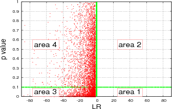
Now we plot p value vs LR as shown in figure 6 for ρ < 0.1. We divide the figure into four areas: area 1, area 2, area 3, and area 4
with green lines as borders to see how sparse the points in each area. Area 1: LR=positive sign and p value < 0.1. Area 2: LR=positive
sign and p value > 0.1. Area 3: LR=negative sign and p value < 0.1. Area 4: LR=negative sign and p value > 0.1. In this
figure, we see that no points lie in area 1 and area 2 (LR=positive sign) instead 58% data lie in area 3 and 42% data
lie in area 4. This figure gives us an explanation that the alternative model is better. Although in the case p value
< 0.1 we reject power-law as the plausible model, the alternative model is still better than the power-law model. These
observations clearly demonstrates that comparing the model to other models is a very complex task in highly dynamic
networks.
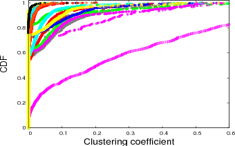
C. Clustering Coefficient
Clustering describes the topology robustness. It has practical implications; for example, if node A is connected to node
B and node B to node C, then there is a probability that node A will also be connected to node C, improving the
robustness of the network against the failure of a connection. Clustering is quantified by a node clustering coefficient as
follows:
 | (5) |
and for the whole graph the clustering coefficient is
 | (6) |
A larger clustering coefficient represents more clustering at nodes in the graph, therefore the clustering coefficient expresses
the local robustness of the network. The distinction between a random and a non-random graph can be measured by
clustering-coefficient metrics [19]. A network that has a high clustering coefficient and a small average path length
is called a small-world model [19]. Newman [20] mentions that virus outbreaks spread faster in highly clustered
networks. In Bittorrent systems, a previous study [21] mentioned the possibility that Bittorrent’s efficiency partly comes
from the clustering of peers. Figure 7 shows the CDF clustering coefficient value of our data sets. The coefficient
clustering values are very sparse showing values. Between 70% and 90% of the clustering coefficient values are under 0.1,
while one data set shows around 40%. This low clustering coefficient observation is the same as that observed by Dale
et al. [16]. Considering only the low clustering coefficient, the Bittorrent topologies seem close to random graphs.
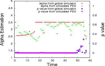
V. Confirmation via Simulation
Here we use simulations to compare the overlay topology properties based on our real-world experiments. We set the maximum peer
set size to 80, the minimum number of neighbors to 20, and the maximum number of outgoing connection to 80. In
our simulation, the result is quite easy to get since we are on a controlled system; we can directly read the global
topology properties from our results. We also have the simulated PEX messages. We compare the global overlay topology
properties as the final result from the simulator with the overlay topology that we get from PEX on the same simulator.
Figure 8 shows the α estimate and p value both for the global result and the PEX result from our simulator. It clearly
shows that global result and the PEX result from the simulator produce very low p values. We calculate the Spearman
correlation for both α values from the global result and the PEX result. The Spearman rank correlation coefficient is a
non-parametric correlation measure that assesses the relationship between two variables without making any assumptions of a
monotonic function. The Spearman rank correlation test gives 0.38 ≤ ρ ≤ 0.5, which we consider to be moderately well
correlated.
VI. Related Work
Bittorrent protocol performance has been explored deeply by several researchers [3] [22] [23] [24]. The rarest first algorithm was
discussed in [22], average download speed was discussed in [23], peer arrival and departure process was discussed in [3],and the
effect of distributon of the peers on the download job progress was discussed in Y.Tian et al. [24]. The huge numbers of peers each
send a P2P download request to a random target on the Internet and anti-P2P companies inject bogus peers through PEX was
discussed in Z.Li et al. [25]. Higher upload-to-download ratios in Bittorrent darknet were discussed in C.Zhang et al.
[26]. Although we know that the topology can have a large impact on performance, to date only a few papers have
addressed the issue. Urvoy et al. [27] used a discrete event simulator to show that the time to distribute a file in a
Bittorrent swarm has a strong relation to the overlay topology. Al-Hamra et al. [28], also using a discrete event simulator,
showed that Bittorrent creates a robust overlay topology and the overlay topology formed is not random. They also show
that peer exchange (PEX) generates a chain-like overlay with a large diameter. Dale et al. [16], in an experimental
study on PlanetLab, show that in the initial stage of Bittorrent a peer will get a random peer list from the tracker.
They found that a network of peers that unchoked each other is scale-free and the node degree follows a power-law
distribution with exponent approximately 2. Dale et al. [16] also showed that the path length formed in Bittorrent
swarms averages four hops and Bittorrent swarms have low average clustering coefficient. However, little work has
been done on determining that topology in the real world. Our results agree with previous research [16] in some
areas and disagree in others, perhaps for two reasons. First, power-law claims must be handled carefully. Many steps
are required to confirm the power-law behavior, including alternative model checking, and we must be prepared for
disappoinment since other models may give a better fit. Second, our methodology relies on real work measurement
combine with simulation for validation. We are using real swarms from a real and operational Bittorrent tracker. This
real world measurement will reflect different type of clients connected to our swarm and each client has a different
behavior. We also face difficult-to-characterize network realities such as NAT and firewalls. Our ability to reproduce key
aspects of the topology dynamics suggests that these factors have only limited impact on the topology, somewhat to our
surprise.
VII. Conclusion and Future Work
We have investigated the properties of Bittorrent overlay topologies from the point of view of the peer exchange protocol using real
swarms from a real and operational Bittorrent tracker on the Internet. We obtain instantaneous snapshots of the active topology of the
Bittorrent network over a month. We cope with the dynamics of the overlay by sampling peer properties. Our results agree in some
particulars and disagree in others with prior published work on isolated testbed experiments on Bittorrent, suggesting that more work is
required to fully model the behavior of real-world Bittorrent networks. Unlike [16], we find that the node degree
of the graph formed in Bittorrent swarm can be described by power law with exponential cut-off and low clustering
observation implies Bittorrent networks are close to random networks. Some areas of improvement that we have identified
for future work are: more correlation analysis number of peers with α and p value, continued characterization with
NATed peers, wider likelihood ratio test with other models and comparing the results with simulation for global graph
properties such as distance distribution and spectrum. We hope to incorporate these properties into a complete dK
series for the evolution of a real-world Bittorrent overlay as it evolves over time [15]. We conclude that further work
throughout the community is necessary to continue to improve the agreement of simulation and controlled experiment with
the real world, and that such work will impact our understanding of Bittorrent performance and its effects on the
Internet.
Acknowledgements
We thank Daniel Stutzbach for help on graph sampling, Aaron Clauset for help on loglikelihood test and power-law Matlab code,
Sue Moon and Joe Touch for suggestions.
References
[1] C. Labovitz, S. Iekel-Johnson, D. McPherson, J. Oberheide, and F. Jahanian, “Internet inter-domain traffic,” ACM SIGCOMM Computer
Communication Review, vol. 40, no. 4, pp. 75–86, 2010.
[2] Cisco Visual Networking Index, “Forecast and methodology, 2009–2014,” White paper, Cisco System, June, vol. 2, 2010.
[3] L. Guo, S. Chen, Z. Xiao, E. Tan, X. Ding, and X. Zhang, “Measurements, analysis, and modeling of Bittorrent-like systems,” in Proceedings of
the 5th ACM SIGCOMM conference on Internet Measurement. USENIX Association, 2005, p. 4.
[4] The Pirate Bay, available on http://www.thepiratebay.org.
[5] C. Zhang, P. Dhungel, and K. Di Wu, “Unraveling the Bittorrent ecosystem,” IEEE Transactions on Parallel and Distributed Systems, 2010.
[6] Bittorrent Client, available on http://en.wikipedia.org/wiki/Comparison_of_BitTorrent_clients.
[7] A. Nordberg, “Rasterbar libtorrent,” available on http://www.rasterbar.com/products/libttorrent.
[8] A. Al-Hamra, N. Liogkas, A. Legout, and C. Barakat, “Swarming overlay construction strategies,” in Computer Communications and Networks,
2009. ICCCN 2009. Proceedings of 18th Internatonal Conference on. IEEE, 2009, pp. 1–6.
[9] D. Stutzbach, R. Rejaie, and S. Sen, “Characterizing unstructured overlay topologies in modern P2P file-sharing systems,” Networking, IEEE/ACM
Transactions on, vol. 16, no. 2, pp. 267–280, 2008.
[10] D. Stutzbach and R. Rejaie, “Understanding churn in peer-to-peer networks,” in Proceedings of the 6th ACM SIGCOMM conference on Internet
measurement. ACM, 2006, pp. 189–202.
[11] D. Stutzbach, R. Rejaie, N. Duffield, S. Sen, and W. Willinger, “Sampling techniques for large, dynamic graphs,” in INFOCOM 2006. 25th IEEE
International Conference on Computer Communications. Proceedings. IEEE, 2007, pp. 1–6.
[12] D. Wu, P. Dhungel, X. Hei, C. Zhang, and K. Ross, “Understanding peer exchange in Bittorrent systems,” in Peer-to-Peer Computing (P2P), 2010
IEEE Tenth International Conference on. IEEE, 2010, pp. 1–8.
[13] A. Clauset, C. Shalizi, and M. Newman, “Power-law distributions in empirical data,” SIAM review, vol. 51, no. 4, pp. 661–703, 2009.
[14] J. Doyle, D. Alderson, L. Li, S. Low, M. Roughan, S. Shalunov, R. Tanaka, and W. Willinger, “The robust yet fragile nature of the internet,”
Proceedings of the National Academy of Sciences of the United States of America, vol. 102, no. 41, p. 14497, 2005.
[15] P. Mahadevan, D. Krioukov, K. Fall, and A. Vahdat, “Systematic topology analysis and generation using degree correlations,” in Proceedings of
the 2006 conference on Applications, technologies, architectures, and protocols for computer communications. ACM, 2006, pp. 135–146.
[16] C. Dale, J. Liu, J. Peters, and B. Li, “Evolution and enhancement of Bittorrent network topologies,” in Quality of Service, 2008. IWQoS 2008. 16th
International Workshop on. IEEE, 2008, pp. 1–10.
[17] M. Mitzenmacher, “A brief history of generative models for power law and lognormal distributions,” Internet mathematics, vol. 1, no. 2, pp. 226–251,
2004.
[18] Q. Vuong, “Likelihood ratio tests for model selection and non-nested hypotheses,” Econometrica: Journal of the Econometric Society, vol. 57, no. 2,
pp. 307–333, 1989.
[19] D. Watts and S. Strogatz, “Collective dynamics of small-world networks,” Nature, vol. 393, no. 6684, pp. 440–442, 1998.
[20] M. Newman, “Properties of highly clustered networks,” Physical Review E, vol. 68, no. 2, p. 26121, 2003.
[21] A. Legout, N. Liogkas, E. Kohler, and L. Zhang, “Clustering and sharing incentives in Bittorrent systems,” in Proceedings of the 2007 ACM
SIGMETRICS international conference on Measurement and modeling of computer systems. ACM, 2007, pp. 301–312.
[22] A. Legout, G. Urvoy-Keller, and P. Michiardi, “Rarest first and choke algorithms are enough,” in Proceedings of the 6th ACM SIGCOMM conference
on Internet measurement. ACM, 2006, pp. 203–216.
[23] J. Pouwelse, P. Garbacki, D. Epema, and H. Sips, “A measurement study of the Bittorrent peer-to-peer file-sharing system,” Delft University of
Technology Parallel and Distributed Systems Report Series, Tech. Rep. Technical Report PDS-2004-007, 2004.
[24] Y. Tian, D. Wu, and K. Ng, “Modeling, analysis and improvement for Bittorrent-like file sharing networks,” in INFOCOM 2006. 25th IEEE
International Conference on Computer Communications. Proceedings. IEEE, 2007, pp. 1–11.
[25] Z. Li, A. Goyal, Y. Chen, and A. Kuzmanovic, “Measurement and diagnosis of address misconfigured p2p traffic,” in INFOCOM, 2010 Proceedings
IEEE. IEEE, 2010, pp. 1–9.
[26] C. Zhang, P. Dhungel, Z. Liu, and K. Ross, “Bittorrent darknets,” in INFOCOM, 2010 Proceedings IEEE. IEEE, 2010, pp. 1–9.
[27] G. Urvoy-Keller and P. Michiardi, “Impact of inner parameters and overlay structure on the performance of Bittorrent,” in INFOCOM 2006. 25th
IEEE International Conference on Computer Communications. Proceedings. IEEE, 2007, pp. 1–6.
[28] A. Al Hamra, A. Legout, and C. Barakat, “Understanding the properties of the Bittorrent overlay,” CoRR abs/0707.1820, 2007.
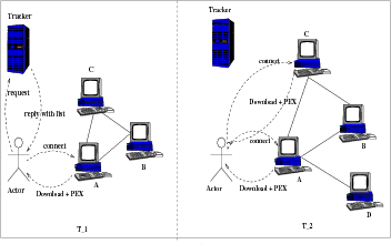 Fig. 1. Simplified view of our approach. Left: At time t=1, the actor gets a PEX message from peer A and learns that peer A is connected to peer B and
C. At t=2, the actor gets PEX messages from peers C and A. The actor learns that now peer A is connected to peer D. Thus the actor knows the properties
of peer A at t=1 and t=2.
Fig. 1. Simplified view of our approach. Left: At time t=1, the actor gets a PEX message from peer A and learns that peer A is connected to peer B and
C. At t=2, the actor gets PEX messages from peers C and A. The actor learns that now peer A is connected to peer D. Thus the actor knows the properties
of peer A at t=1 and t=2.